Planning capacity for an LLM server on Intel Arc Pro

NoteHow to read the examples

This article explains a capacity-planning method. Symbols and normalized values in the examples and figures are deliberately illustrative. They are not benchmark results for Qwen3.8, Intel Arc Pro, SGLang, or the container image.

I write request sizes as input/output tokens, so 8K/1K means 8,192 input tokens followed by 1,024 requested output tokens. Those dimensions define workloads; they do not disclose throughput, latency, or capacity.

Peak output throughput does not tell me how many requests I can safely admit. The decoder can remain busy while new prompts spend their first-token budget in a queue. A large token pool can sit partly empty while a hybrid model has no recurrent-state slot for another sequence. A larger tensor-parallel group can improve one request and still lose total capacity to two smaller replicas.

Capacity is the intersection of four things:

1. a declared workload and arrival process;
2. a vector of latency and correctness objectives;
3. a complete serving topology and resource profile;
4. a repeatable rule for deciding where the passing region ends.

That definition gives me two boundaries, not one. I first want the laboratory saturation boundary: how many outstanding requests this fixed server can carry before one of its contracts fails. Closed-loop concurrency is efficient for finding it. I then want the production admission boundary: what offered arrival process the deployment can absorb without an ever-growing queue. Open-loop rate tests and trace replay answer that second question.

The concrete system in this post is Qwen3.8-27B on four Intel Arc Pro B70s. It is a dense hybrid model, split with tensor parallelism and served through SGLang. Its MTP head proposes tokens before the target verifies them. I use that server to make every step runnable, but I keep measured Arc Pro results out of the article. The point is the method: build a model, make one controlled change, inspect the right artifact, and let that evidence choose the next experiment.

AIPerf is the load generator and evidence recorder in this workflow. It cannot decide what the workload means, whether the server selected the intended kernel, which memory pool is binding, or whether a closed-loop result survives real arrivals. Those are capacity-planning decisions.

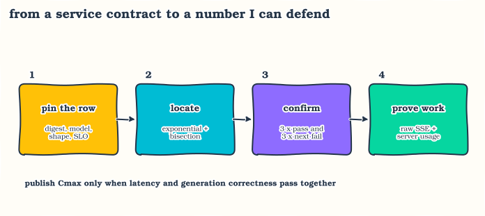
Figure 1. Capacity planning is a loop from workload to operating policy, not a benchmark command followed by one number.

Part I: Make one request boringly reproducible

Pin the image and model

Tags can move, so I resolve the public image tag to an immutable digest before the first run:

docker pull rahulunair/sglang-xpu:qwen3.8-27b
docker image inspect rahulunair/sglang-xpu:qwen3.8-27b \
  --format '{{index .RepoDigests 0}}'

I record the returned digest in an experiment manifest and do the same for the model snapshot. I used ulkaa/Qwen3.8-27B-AWQ-INT4, an activation-aware weight-quantized W4A16 checkpoint with four-bit weights and 16-bit activations. Its BF16 MTP head supplies the speculative draft, so it does not require a second model directory.

The public rahulunair/sglang-xpu recipe is the starting point. This template keeps the settings that matter to the capacity investigation visible. Substitute the digest recorded locally:

: "${IMAGE:?set IMAGE to a pinned rahulunair/sglang-xpu digest}"
: "${MODEL_DIR:?set MODEL_DIR to the pinned checkpoint snapshot}"
: "${CONTAINER:?choose a local container name}"

SERVER_ARGS=(
  python -m sglang.launch_server
  --model-path /model --served-model-name Qwen3.8-27B
  --device xpu --tp-size 4 --host 0.0.0.0 --port 30000
  --trust-remote-code --attention-backend intel_xpu --page-size 64
  --context-length 12288 --max-total-tokens 262144
  --chunked-prefill-size 4096 --mem-fraction-static 0.85
  --max-running-requests 64 --max-mamba-cache-size 128
  --disable-custom-all-reduce --watchdog-timeout 1800
  --cuda-graph-config '{"decode":{"backend":"full","bs":[1,2,4,8,12,16,20,24,25]},"prefill":{"backend":"disabled"}}'
  --skip-server-warmup --language-only --enable-cache-report --enable-metrics
  --reasoning-parser qwen3 --tool-call-parser qwen3_coder
  --strip-thinking-cache --enable-strict-thinking
  --speculative-algorithm EAGLE --speculative-num-steps 7
  --speculative-eagle-topk 1 --speculative-num-draft-tokens 8
)

The launch then binds the device nodes, model snapshot, and the resolved image digest. I keep the model mount read-only:

docker run -d --name "$CONTAINER" \
  --device=/dev/dri -v /dev/dri:/dev/dri \
  --group-add video --group-add "$(getent group render | cut -d: -f3)" \
  --ipc=host --shm-size=64g \
  --cap-add=SYS_PTRACE --security-opt seccomp=unconfined \
  --ulimit memlock=-1 --ulimit stack=67108864 \
  -p 30000:30000 -e ONEAPI_DEVICE_SELECTOR=level_zero:gpu \
  -e XPU_REPO=/opt/xpu -e XPU_DENSE_INT8_MAX_M=8 \
  -e XPU_SYMM_AR_MAX_BYTES=131072 \
  -v "$MODEL_DIR:/model:ro" \
  "$IMAGE" "${SERVER_ARGS[@]}"

Check readiness without generating or warming the path under test:

curl -fsS http://127.0.0.1:30000/health
curl -fsS http://127.0.0.1:30000/v1/models | jq
docker logs "$CONTAINER" 2>&1 | rg -m1 'server_args=ServerArgs'
docker logs "$CONTAINER" 2>&1 | rg 'max_total_num_tokens' | tail -1

Save the identity before saving a result

A digest is necessary and still not enough. My manifest also includes the model revision, AIPerf version, SGLang revision exposed by the image, full resolved server arguments, device selection, driver and runtime versions, client host, network path, topology, prompt-corpus hash, cache policy, random seed, and start and end timestamps. If one of those changes, I have a new experiment.

This is the shape of the manifest I keep beside the raw artifacts:

: "${RUN_DIR:?set a new artifact directory}"
: "${MODEL_DIR:?set the pinned model snapshot}"
: "${IMAGE:?set the immutable image reference}"

mkdir -p "$RUN_DIR"
{
  printf 'utc_start=%s\n' "$(date -u +%FT%TZ)"
  printf 'image=%s\n' "$IMAGE"
  printf 'model_tree=%s\n' "$(git -C "$MODEL_DIR" rev-parse HEAD 2>/dev/null || true)"
  printf 'aiperf=%s\n' "$(aiperf --version)"
  printf 'kernel=%s\n' "$(uname -r)"
  docker image inspect "$IMAGE" --format '{{json .RepoDigests}}'
  docker inspect "$CONTAINER" --format '{{json .Config.Cmd}}'
} > "$RUN_DIR/manifest.txt"

The exact model snapshot may not be a Git checkout, so in a formal harness I hash its revision metadata and selected configuration files instead. I also save the generated request corpus. A seed without the tokenizer, template, and generator version is not a reproducible workload.

Before loading the server, I check the client side as well. The load generator needs enough workers, file export must keep up, and the network path must not be the first bottleneck. A client CPU at full utilization or a semaphore that never reaches the requested load means I measured the harness. I retain actual issued request rate, achieved concurrency, client errors, and worker occupancy beside server-side queue and cache metrics.

Part II: Turn traffic into a workload model

Start with a trace record, not an average prompt

The runnable anchor in this post uses a fixed input/output shape. That is useful for isolating mechanisms, but a production model begins one level earlier. For each request I want at least:

arrival timestamp
templated input length
requested and actual output length
session and turn identifier
shared-prefix identity or reusable-prefix length
streaming mode
tool-call or structured-output marker
finish reason, cancellation, and error
latency objective class

I derive a few workload classes from that trace: short interactive turns, long-prefill requests, long-decode requests, multi-turn sessions with prefix reuse, tool or structured-output requests, and background work. The labels are less important than preserving the relationships in the data.

A mean input length and mean output length erase the expensive part. Input and output can be correlated. Long sessions can have more prefix reuse than short ones. Tool calls can return early, then arrive again with a larger prompt. Burstiness can differ by class. If I sample every column independently, I may create requests that never occur and omit the combinations that dominate the tail.

For diagnosis I still use exact shapes such as 8K/1K. They turn a fuzzy traffic mix into a controlled probe. I write those probes as \(W_{short}\), \(W_{prefill}\), and \(W_{decode}\) and preserve the deployment’s observed class shares. For the production qualification I replay the paired shapes and arrival timestamps, or use an empirical distribution that preserves their covariance. AIPerf supports fixed schedules and several rate-driven modes; its official timing-mode reference is worth reading before combining --request-rate and --concurrency.

The contract is a vector

TTFT protects prompt admission and prefill waiting. It says nothing about the cadence after streaming begins. TPOT or inter-token latency protects that decode experience. End-to-end latency protects completion of the whole request. Error, cancellation, finish-reason, and output-length gates stop a fast failure from becoming a good result.

For workload class \(w\), I write the contract as:

\[ S(w)=\{T_{TTFT}, T_{TPOT}, T_{E2E}, E_{max}, V_{output}\}. \]

The symbols mean locally chosen thresholds and a validity predicate, not values borrowed from another deployment. A request contributes to goodput only when it satisfies every applicable latency condition and produces a valid response. At offered rate \(\lambda\):

\[ G(\lambda,w)=\lambda \cdot P\!\left(\text{all SLO and validity gates pass}\mid w\right). \]

The operational capacity I eventually want is therefore:

\[ \lambda_{edge}(W,S)=\sup\{\lambda:G(\lambda,W)\text{ meets the declared attainment target}\}. \]

\(W\) includes the joint request and arrival distribution, and \(S\) is the whole contract vector. This is an offered-load boundary. It is deliberately separate from closed-loop \(C_{edge}\).

That is the useful interpretation of goodput in DistServe: the rate of requests that remain inside their per-request objectives, not the raw rate at which the server emits tokens. DistServe also makes the prefill/decode separation explicit. Those phases can require different parallelism and can interfere when they share a device.

For the fixed-shape closed-loop probe, I use the simpler boundary:

\[ C_{edge}(w)=\max\{C:\text{every confirmation at }C\text{ passes }S(w)\}. \]

I test the adjacent integer too. If the higher point is mixed across confirmations, I do not average it into a pass.

Choose the arrival process deliberately

mode	what it holds fixed	question it answers	main trap
closed loop	outstanding requests	where this server saturates	slower completions automatically reduce offered rate
open loop	scheduled arrivals	whether an arrival rate is stable	the queue can grow before requests fail
rate plus concurrency cap	arrival process and client safety ceiling	how a bounded client population behaves	the cap adds client-side backpressure
fixed schedule	exact trace timestamps	whether a captured event or traffic window replays	it qualifies only that trace and scale factor

In closed loop, a completion releases a client slot and immediately creates the next request. When service slows, replacement slows too. In open loop, arrivals continue according to the schedule and waiting work can accumulate. This is why I use closed loop to locate the interesting region and open loop to decide whether the region can carry production traffic.

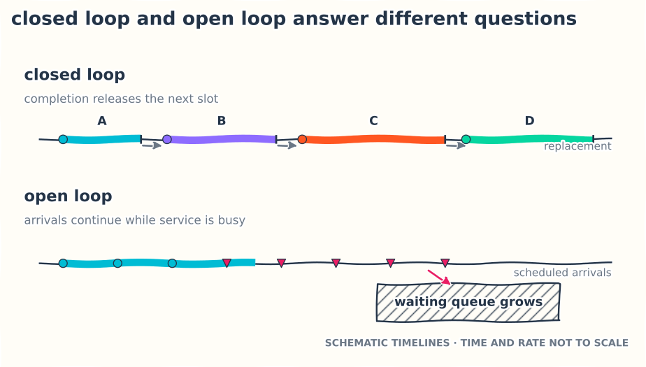
Figure 2. Closed loop discovers saturation efficiently; open loop exposes queue stability under offered traffic.

Little’s Law, \(L=\lambda W\), is useful intuition here: more arrival rate or more time in the system implies more work in flight. It is not my capacity calculator. Continuous batching, prompt/decode interference, cache hits, variable output length, admission policy, and tail objectives make the service process state-dependent. I use the identity to catch impossible stories, then measure the real scheduler.

AIPerf can generate constant, Poisson, and gamma arrivals. A Poisson label does not make a workload realistic, and a gamma smoothness setting should come from traffic or be declared as a stress case. Its arrival-pattern documentation explains the scheduling mechanics. My capacity record says which process was used and why.

Part III: Model the server before searching it

Begin with a memory ledger

The first topology must fit before it can be fast. I split device memory into terms that behave differently:

\[ M_{used}=M_{weights}+M_{runtime}+M_{graphs}+M_{token\ state}+M_{sequence\ state}+M_{headroom}. \]

Tensor parallelism usually shards a large fraction of the weights, but not every buffer follows the same rule. Graph workspaces can grow with captured batch shapes. Attention KV grows with resident tokens. A recurrent or hybrid model can carry a fixed state allocation per active sequence. The allocator’s startup report is evidence; dividing nominal device memory by parameter count is only a first estimate.

Qwen3.8-27B makes that distinction concrete. It is dense, so each token uses the same feed-forward weights. Of its 64 decoder layers, 16 use full attention and 48 use Gated DeltaNet. Full-attention layers append key and value pages as a sequence grows. Gated DeltaNet layers retain fixed-shape recurrent state for each active sequence. SGLang calls the latter its Mamba cache machinery even though these model blocks are Gated DeltaNet.

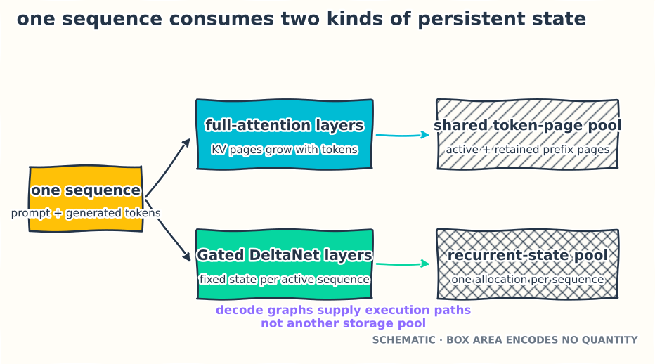
Figure 3. Token-indexed state and sequence-indexed state create different capacity ceilings.

For a dense attention model, a first-order memory ceiling is often dominated by weight residency and KV pages. For this hybrid model I need both:

\[ C_{state}=\left\lfloor\frac{R}{e}\right\rfloor, \qquad C_{tokens}\text{ such that }\sum_i L_i\leq P. \]

\(R\) is the recurrent-state pool, \(e\) is the number of entries consumed per active request under the pinned allocator policy, \(P\) is the shared token pool, and \(L_i\) is the resident token footprint of request \(i\). I read \(e\) from the runtime behavior. I do not copy it from another hybrid model or assume it from a flag name.

The important server arguments map to those objects:

flag	controlled object	what it does not mean
--context-length	admission ceiling for one templated prompt plus output	it does not reserve that length for every request
--max-total-tokens	shared token-page storage for active and cached sequences	it is not the maximum number of active requests
--max-running-requests	requested scheduler ceiling	the resolved runtime may lower it
--max-mamba-cache-size	recurrent-state entries for hybrid sequences	it is not ordinary attention KV capacity
decode graph batch list	captured execution shapes	it is not an admission limit
--chunked-prefill-size	prompt scheduling granularity	it does not remove prompt compute
--page-size	allocation and attention paging granularity	a smaller page is not automatically faster

I save the resolved allocation line and graph-capture completion from every server start. A configuration file records what I asked for. The log records what I got.

Model prefill and decode separately

Prefill processes prompt tokens in parallel and is commonly compute-heavy. Decode advances one position per active sequence and commonly puts more pressure on weight movement, cache access, small kernels, and collectives. The exact balance changes with batch, context, architecture, quantization, and hardware.

Orca established iteration-level scheduling as the practical way to reform a batch as sequences finish and new work arrives. That means “batch size” is not one static property of a request. It changes through prefill and every decode iteration, which is why I retain batch composition rather than attach one throughput value to a model.

The Sarathi-Serve paper is useful here because it treats chunked prefill as a scheduling tool for controlling prefill/decode interference, not as a magic reduction in prompt work. The PagedAttention paper explains why paged KV management improves how many variable-length sequences can share device memory. The SGLang paper adds prefix-aware RadixAttention, which makes cache state and request similarity part of the workload.

I build three small curves before searching capacity:

1. Prefill curve: fixed output, varied input, concurrency one. This shows how TTFT changes with prompt length and whether chunk boundaries or attention kernels create discontinuities.
2. Decode curve: fixed input, varied output and active batch. This shows TPOT, graph-bucket transitions, and state growth while keeping prompt work bounded.
3. Residency curve: fixed request shape, varied active sequences and retained prefixes. This exposes token-page, recurrent-state, and graph limits.

These are navigation probes. They tell me which full-server experiment is worth running. AIPerf includes prefill-ttft-curve, decode-itl-curve, and concurrency-ramp recipes in its search documentation, but the same curves can be built manually when I need tighter control over cache or server lifecycle.

For a larger topology space, I fit an interpolated cost model from those operator and full-iteration probes and replay the workload in a simulator. The Vidur paper is the useful precedent: profile the operations, model the runtime, simulate candidate configurations, then validate the finalists on hardware. I use the model to prune bad candidates, not to publish an unmeasured capacity. Large prediction error is itself a result: it sends me back to a missing collective, cache regime, scheduler transition, or state constraint.

Select topology before tuning small flags

The tempting rule is “increase TP until TTFT passes, then add DP.” I use a more careful version:

1. Find the smallest TP group that fits the weights, required context, graph memory, and state pools with real headroom.
2. Measure one request and the representative latency curves at each feasible TP.
3. Reject any topology that fails correctness, backend reachability, or a per-request latency objective.
4. At a fixed total device budget, compare one larger TP group against more replicas built from the smallest qualified TP group.
5. Measure the winning candidates again under open-loop and mixed traffic.

More TP shards one request across more devices. It may be required for fit and can reduce per-rank work, while adding collective communication and using devices that could have formed another replica. Ordinary data parallelism makes independent model replicas. It gives each replica its own scheduler and cache, then adds routing, imbalance, and cache-locality decisions outside the model.

For four devices, the design table is simple even when the answer is not:

one TP4 replica
two TP2 replicas behind a router
four TP1 replicas, only if TP1 passes the fit and latency gates

The total-device comparison is the key. TP4 versus TP2 on different device budgets answers a latency scaling question. One TP4 replica versus two TP2 replicas on the same four devices answers a capacity-planning question.

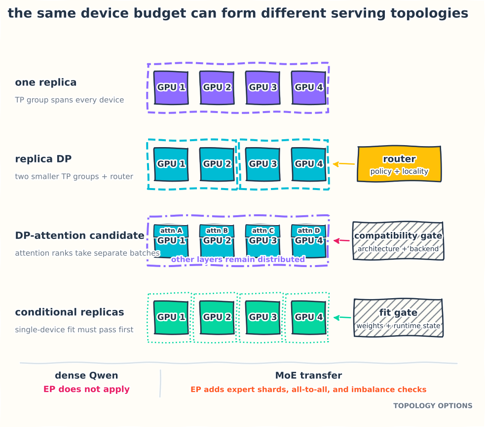
Figure 4. TP, replica DP, DP-attention, and EP solve different problems. I do not put them on one slider.

With multiple replicas, I retain per-replica request counts, queued tokens, cache-hit state, errors, and latency. A round-robin router can balance requests and destroy prefix locality. A cache-aware router can preserve reuse and create a hot replica. A capacity claim for replicas includes the routing policy. SGLang’s current DP, DP-attention, and Model Gateway guide documents these modes and their launch shapes.

DP-attention is not ordinary DP

SGLang’s DP-attention lets attention process independent request batches across DP ranks while other parts of the model retain distributed execution. In the current server-argument contract, TP size is the overall distributed world and must be divisible by DP size; enabling DP-attention also changes internal attention groups and chunked-prefill handling. That is materially different from placing complete independent replicas behind a gateway.

DP-attention is especially relevant to architectures where attention and MoE feed-forward layers want different parallel layouts. It is not a free capacity switch. Before measuring it on a new model/backend combination, I require:

• startup shows the intended DP and attention-TP groups;
• one-request greedy output matches the control topology;
• several simultaneous streams return the expected records and lengths;
• KV and recurrent state remain request-local;
• radix reuse and cache flush behave correctly;
• the intended attention, collective, and MoE paths actually serve;
• no rank starves while another rank owns most of the queue.

Qwen3.8 adds hybrid recurrent state and MTP to that compatibility surface. A flag being accepted does not prove this exact XPU path is supported. If a gate fails, my result is “not qualified for this stack,” not a performance verdict.

EP is a branch for MoE models

Qwen3.8-27B is dense. It has no routed feed-forward experts, so expert parallelism is not a tuning axis for this server.

For an MoE model, EP shards expert weights and routes token representations to the ranks that own the selected experts. That makes dispatch, expert grouped GEMMs, combine, and expert imbalance part of the critical path. The slow rank can set the layer time even when average token counts look balanced. Prefill and decode may prefer different communication modes because their message shapes and latency tolerance differ.

SGLang exposes --ep-size, --moe-a2a-backend, --moe-runner-backend, and Expert Parallelism Load Balancing. Its official expert-parallelism guide also records backend constraints: several all-to-all backends require EP size to equal the overall TP world, while hybrid TP/EP may fall back to a different dispatch path. I treat those as versioned compatibility rules and read the pinned runtime before designing the sweep.

My MoE capacity record adds:

tokens routed to each expert and rank
experts activated per rank
dispatch and combine time
grouped-GEMM shape distribution
overflow, drop, or padding behavior
expert placement and redundant experts
load-balancer observation and rebalance windows
network topology and cross-node traffic

The MegaScale-Infer paper goes further and disaggregates attention from expert FFNs so each can scale independently. I do not begin there. I first establish TP and EP behavior on one declared topology, then add DP-attention, load balancing, overlap, or disaggregation one mechanism at a time. Otherwise an all-to-all improvement, a routing-distribution change, and a scheduler change become one uninterpretable result.

Consider prefill/decode disaggregation only after locating interference

If TTFT and TPOT cannot both meet their objectives on a colocated server, prefill/decode disaggregation becomes a topology candidate. DistServe and Splitwise show why: prompt processing and token generation have different resource profiles, so their replica counts and parallelism can be planned separately. The cost is KV transfer, routing, another queue, and another failure domain.

I add disaggregation after the single-server curves tell me prefill/decode interference is material. Then the capacity model includes prefill goodput, decode goodput, transfer bandwidth and tail, queue balance between stages, and the placement of both pools. A fast prefill tier that overwhelms decode is not a balanced deployment.

Part IV: Define cache and warmup state

“Warm” needs three nouns

Kernel compilation, graph capture, allocator state, and radix contents are different. I use three explicit protocols:

protocol	engine and graphs	prefix cache	purpose
cold process	newly started	empty	startup and first-use study, kept outside steady-state capacity
warm engine, cold cache	required paths exercised	flushed before measurement	conservative unique-prompt boundary
warm engine, representative cache	required paths exercised	seeded with the declared reuse distribution	production cache behavior

--skip-server-warmup controls SGLang’s startup action. It does not remove the need for a load-test warmup. A serial warmup also does not exercise every graph bucket or scheduler shape, so I verify graph capture in the log and issue a separate shape warmup when the runtime requires it.

Warmup prompts must be disjoint from the measured set in a cold-cache test. I learned this the annoying way. A small synthetic corpus reused warmup entries in the measured phase. Radix hits then made a few first-token observations look excellent even though the protocol was supposed to measure cold unique prompts. The median remained usable for a smoke test, but the run was invalid as capacity evidence.

A common chat template can still create reusable prefixes when prompt bodies are unique. I therefore retain the server’s cached-prompt-token report for each request, not merely prompt hashes. Cold-cache and representative-cache results are separate workload definitions. I never average them together.

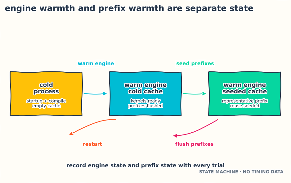
Figure 5. Warm kernels and warm prefixes answer different questions.

Administrative actions can change the system

I use /health for readiness, not a generation endpoint. A generation health probe compiles shapes, allocates state, and seeds caches. It is workload.

/flush_cache is also not innocent on every experimental path. A cache flush touches scheduler and allocator lifecycle, and I have found speculative paths where an administrative flush exposed a graph-lifetime defect that ordinary multi-turn traffic did not. The harness checks the flush response, waits for the server to become healthy, and runs a small lifecycle canary before trusting the next trial. If the production path never flushes cache, I still fix or scope the defect, but I do not confuse it with normal request behavior.

Part V: Use controlled probes to find the binding resource

The manual campaign that mattered

The decisive capacity work was the sequence of failed explanations before the final search.

I first lowered only the per-request context ceiling while keeping the physical token pool, recurrent-state budget, and graph list unchanged. The short-workload boundary did not move. That ruled out the story that maximum context was reserving its full length for every request.

I then changed the shared token pool at a fixed tested concurrency. The qualitative outcome stayed the same. Token pages were not binding in that region.

Next I enlarged the recurrent-state pool and extended decode graph coverage to the newly reachable active batch shapes. The short-workload envelope moved. A separate longer-prompt probe did not. That split the mechanism cleanly: the short workload had reached a state/graph ceiling, while the longer workload had spent its first-token budget in prefill before that ceiling mattered.

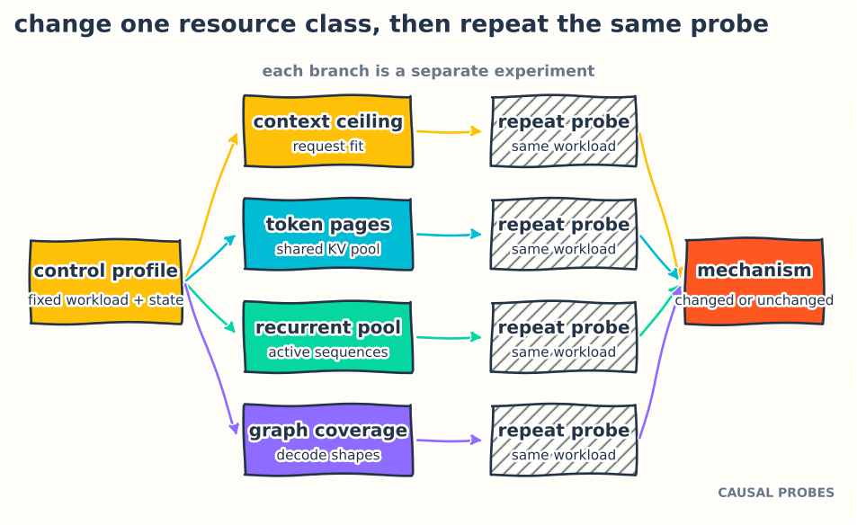
Figure 6. One resource class per branch turned a capacity result into a mechanism.

I cannot assign the short-workload change separately to recurrent entries and new graph buckets because those two must form a usable profile together. I can say the old active-sequence ceiling was real, the context-only theory was wrong, and the longer workload was constrained elsewhere. That is enough to choose the next experiment.

Read latency as a fingerprint, not a diagnosis

observation	likely class	next controlled probe
TTFT rises while TPOT stays stable	prefill queue or admission pressure	vary input length, chunk policy, and open-loop rate
TTFT stays stable while TPOT rises	decode saturation, communication, or graph gap	inspect active batch and graph coverage
both rise	scheduler backlog or broad saturation	lower admitted work and inspect queue depth
short prompts improve, long prompts do not	prefill-bound long path	build a prefill curve and inspect final chunks
active requests stop below configured ceiling	memory, recurrent state, or allocator policy	read resolved pools and per-request state use
one replica degrades	router imbalance or cache locality	inspect per-replica queues and prefix hits
periodic outliers	compilation, host stall, device state, or maintenance	correlate client, server, and device timelines
shortened output, error, or cancellation	invalid trial	discard it before latency analysis

These are hypotheses. For example, a Python stack sampled in a wait function may be waiting for device work rather than causing it. A graph-side fast path may replay without updating a Python counter. I use controlled removal or a path-specific log to establish causality, then repeat the whole-server request.

Throughput can hide the boundary

Consider the invented scenario in Figure 7. TTFT is divided by its local SLO, so the contract boundary is one. Output throughput is divided by a local reference. The adjacent points overlap in throughput even though one side fails first-token latency.

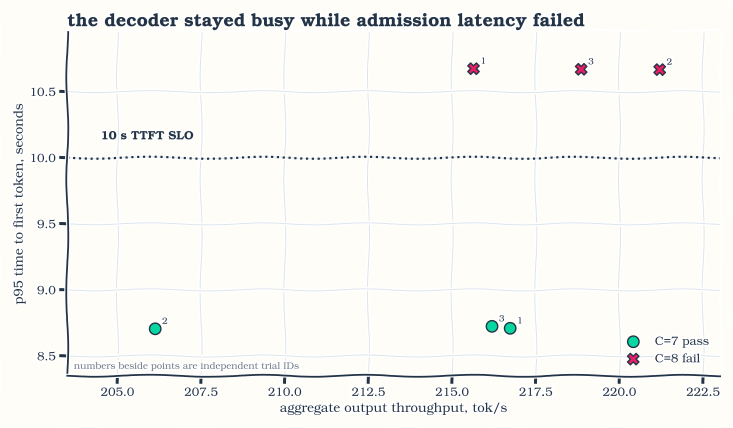
Figure 7. Busy decode is not proof that new prompts are being admitted on time.

Peak tokens per second divided by an average request size ignores queueing, batch composition, and phase interference. It can be a sanity bound. It is not the admission limit.

Part VI: Use AIPerf as an evidence pipeline

Pin the tool and inspect the expanded workload

The retained experiment used AIPerf 0.10.0. At the time of this revision, the official project had moved to 0.12.0. I do not retroactively assign new search or metric semantics to the old evidence. The commands below match the retained release; for a new campaign I pin the executable and read the documentation at that revision. AIPerf evolves quickly, including search defaults and SLO units.

For a longer-lived campaign I prefer a checked-in YAML configuration because a large command is hard to review. AIPerf’s configuration and distribution guides show how to validate and expand configurations. Before any GPU run, I inspect the expanded cells and generated inputs. That catches accidental Cartesian products, missing stop conditions, and an empirical distribution that was silently replaced by independent samples.

For a new 0.12.x campaign, this is the compact open-loop skeleton I start from. The values come from environment variables so the reviewed file describes the experiment without embedding a local capacity result. This version is complete for an unauthenticated local endpoint; the marked line is where I add optional deployment authentication when it is required:

schemaVersion: "2.0"

benchmark:
  model: "${MODEL_NAME}"
  endpoint:
    url: "${INFERENCE_URL}"
    path: /v1/chat/completions
    type: chat
    streaming: true
    timeout: "${REQUEST_TIMEOUT}"
    useServerTokenCount: true
    # ... optional deployment authentication goes here

  tokenizer:
    name: "${TOKENIZER}"
    trustRemoteCode: true

  dataset:
    type: synthetic
    entries: "${DATASET_ENTRIES}"
    prompts:
      isl: {mean: "${ISL}", stddev: 0}
      osl: {mean: "${OSL}", stddev: 0}

  phases:
    - name: warmup
      type: concurrency
      excludeFromResults: true
      requests: "${WARMUP_REQUESTS}"
      concurrency: 1
    - name: profiling
      type: poisson
      rate: "${OFFERED_RATE}"
      concurrency: "${SAFETY_CEILING}"
      duration: "${DURATION}"
      gracePeriod: "${GRACE_PERIOD}"

  slos:
    time_to_first_token: "${TTFT_LIMIT}"
    inter_token_latency: "${ITL_LIMIT}"
    request_latency: "${E2E_LIMIT}"

  artifacts:
    dir: "${ARTIFACT_DIR}"
    summary: [json]
    records: [jsonl]

  gpuTelemetry:
    enabled: false

I run aiperf config validate campaign.yaml, then aiperf config expand campaign.yaml --full, then aiperf profile --config campaign.yaml. For diagnostic pairs of fixed input and output lengths, a YAML zip sweep keeps the pairs together. The default grid would create every cross-product. For a production mix I use saved records or a fixed schedule so session, prefix, length, and arrival relationships survive.

useServerTokenCount keeps the request record aligned with the server’s token accounting. I disable AIPerf’s default GPU telemetry here because the 0.12.0 collectors cover NVIDIA DCGM and AMD SMI, not Intel XPU. Server-side SGLang and device metrics are collected separately and joined to the client timeline.

I still begin with one CLI anchor because it is easy to compare with the server logs:

aiperf profile \
  --model Qwen3.8-27B --url http://127.0.0.1:30000 \
  --endpoint-type chat --streaming --use-server-token-count \
  --tokenizer "$MODEL_DIR" --tokenizer-trust-remote-code \
  --isl "$ISL" --isl-stddev 0 --osl "$OSL" --osl-stddev 0 \
  --extra-inputs '{"temperature":0,"ignore_eos":true}' \
  --random-seed "$SEED" \
  --num-dataset-entries "$((REQUESTS + WARMUPS))" \
  --warmup-request-count "$WARMUPS" --warmup-concurrency 1 \
  --request-count "$REQUESTS" --concurrency "$C" \
  --export-level raw --artifact-dir "$OUT" --ui None \
  --max-workers "$REQUESTS"

Every flag has an experimental meaning:

• fixed ISL/OSL and zero standard deviation isolate one workload cell;
• streaming exposes TTFT and inter-token timing;
• server token counts avoid relying only on retokenized text;
• ignore_eos forces the requested decode work for saturation testing;
• separate dataset entries prevent warmup/profile overlap;
• raw export preserves request and SSE evidence;
• enough workers stop the client pool from becoming the concurrency ceiling.

When SGLang runs with --enable-metrics, I collect its /metrics endpoint with the trial. The useful signals include running and queued requests, token-pool usage, prefix-cache hit rate, generation activity, and request phase histograms. With DP-attention, SGLang requires metrics from every scheduler to see all DP ranks. A client percentile without server queue and occupancy state can show where the boundary is, but not why it exists.

ignore_eos deliberately generates beyond the model’s natural stopping point. That is useful load and not a model-quality evaluation. I run semantic canaries with normal EOS separately.

Use recipes to navigate, not certify

The max-concurrency-under-sla recipe can locate the range between the last observed pass and first failure:

aiperf profile \
  --model Qwen3.8-27B --url http://127.0.0.1:30000 \
  --endpoint-type chat --streaming --use-server-token-count \
  --tokenizer "$MODEL_DIR" --tokenizer-trust-remote-code \
  --isl "$ISL" --isl-stddev 0 --osl "$OSL" --osl-stddev 0 \
  --extra-inputs '{"temperature":0,"ignore_eos":true}' \
  --random-seed "$SEED" --num-dataset-entries "$DATASET_SIZE" \
  --warmup-request-count "$WARMUPS" --warmup-concurrency 1 \
  --request-count "$REQUESTS" \
  --search-recipe max-concurrency-under-sla \
  --ttft-sla-ms "$TTFT_SLO_MS" \
  --concurrency-min "$C_MIN" --concurrency-max "$C_MAX" \
  --search-style monotonic --num-profile-runs 1 \
  --export-level records --artifact-dir "$SEARCH_OUT" \
  --ui simple --max-workers "$C_MAX"

The official sweep guide describes the bundled search questions. I choose the search style from the response surface:

• monotonic brackets and narrows quickly when increasing load produces a clean progression;
• a smoothed isotonic search is useful when noise creates small local reversals around an otherwise monotone boundary;
• a grid is transparent when the candidate range is already small;
• broader Bayesian tuning is useful for many interacting knobs, not necessary for certifying adjacent concurrency values.

Search points can share client process state, corpus entries, and server cache history. That is convenient for navigation and too weak for the final claim. I do not promote search_history directly into a capacity record.

Current AIPerf also supports conjunctive TTFT, TPOT or ITL, end-to-end, and error-rate filters in the concurrency recipe. That is preferable to a TTFT-only search when the product constrains both phases. I still inspect the exact metric, statistic, operator, and unit in the pinned version. Named error-rate flags and generic metric expressions have not always used the same input unit.

For decision-grade tails, the current project recommends multiple profile runs and pooled per-request percentiles rather than averaging run percentiles. That is useful during search. My adjacent certification remains stricter: each independent run must pass its own declared gates, and the raw records must be valid.

Follow the concurrency search with offered load

After certification I sweep a narrow band of scheduled request rates around the candidate region. The concurrency value here is only a high safety ceiling on client connections:

aiperf profile \
  --model Qwen3.8-27B --url http://127.0.0.1:30000 \
  --endpoint-type chat --streaming --use-server-token-count \
  --tokenizer "$MODEL_DIR" --tokenizer-trust-remote-code \
  --request-rate "$RATE" --arrival-pattern poisson \
  --concurrency "$SAFETY_CEILING" \
  --benchmark-duration "$DURATION" \
  --benchmark-grace-period "$GRACE" \
  --export-level raw --artifact-dir "$OUT" --ui None

For every rate I compare scheduled and issued arrivals, queue growth over time, completion after the issuance window, goodput, and every SLO component. A flat completion rate with a growing queue is overload, even if the final requests eventually succeed. I then replay the real or scaled fixed schedule, because a Poisson sweep does not preserve a production burst.

AIPerf’s --prefill-concurrency can be useful for a memory-safe diagnostic. It releases its special slot at the first token, so it self-throttles and can create coordinated omission. I do not use it to qualify production latency.

The AIPerf limitations I design around

These are the parts of the experiment that still belong to the operator.

1. Closed loop applies backpressure. As requests slow, the achieved arrival rate falls. Follow with open-loop rate or trace validation.
2. Search history is stateful. Adaptive points can inherit caches, compiled shapes, or dataset reuse. Re-run final cells in independent processes.
3. Aggregate output can hide invalid requests. Validate raw records, SSE content, finish reasons, errors, and server token usage before reading tails.
4. A synthetic corpus can overlap warmup. Allocate disjoint entries and inspect cache-hit telemetry.
5. Retokenized text is not always the server’s token count. Retain server usage while also checking that substantive text streamed.
6. A single SLO recipe is not a full product contract. Confirm TTFT, TPOT or ITL, end-to-end latency, error, and validity together.
7. The client can be the bottleneck. Check workers, achieved load, CPU, network, export overhead, and timeouts.
8. A fixed marginal distribution can destroy real pairings. Preserve ISL/OSL, session, prefix, and arrival correlations in scenario or trace data.

AIPerf’s request-rate plus concurrency guide is particularly important: the rate schedules attempts, while concurrency is a semaphore ceiling, and there is no catch-up burst after blocked requests. That mechanism must match the client behavior I intend to model.

Part VII: Search, certify, and explain the boundary

Phase A: bracket

I start at a clearly passing load and grow concurrency geometrically until a failure appears. Every point gets its own artifact directory. I save the last pass and first fail, plus the failure reason. If the server errors or the client cannot generate the intended load, I stop and fix validity before narrowing.

Phase B: narrow

I bisect the integer range, or let AIPerf’s monotonic search do it. The purpose is to find neighboring candidates cheaply. A surprising local reversal triggers a repeat and state audit, not an immediate claim that the system is nonmonotone.

Phase C: certify adjacent values

For candidate \(C\) and its next integer:

1. launch a new AIPerf process and artifact directory for every confirmation;
2. establish the declared engine and cache state;
3. use disjoint warmup and measured prompts;
4. rotate seed, prompt order, and the order of the two candidate cells;
5. preserve the same model, server, workload, and SLO vector;
6. validate each raw run before using its latency metrics;
7. require every \(C\) trial to pass and retain every \(C+1\) outcome.

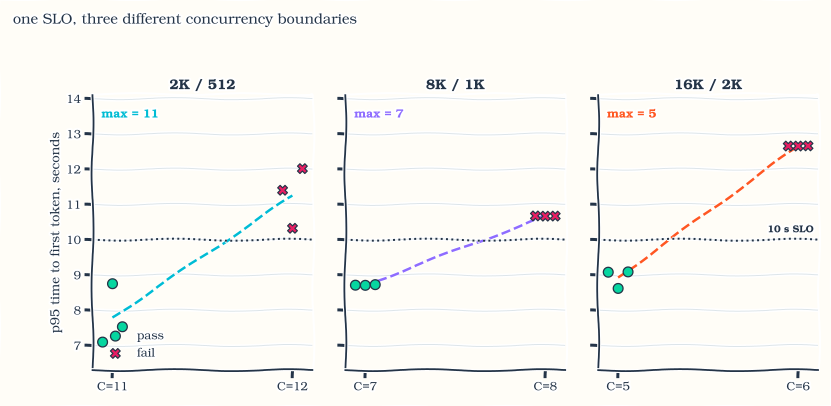
Figure 8. Search finds candidates; independent adjacent trials certify the edge.

I do not average the p95 values from several trials and compare that average to the SLO. An average of percentiles is not the percentile of the pooled request population, and it can conceal a failing run. I keep per-run verdicts, a pooled request view when statistically appropriate, and confidence reporting as separate artifacts. AIPerf’s multi-run guidance is a useful starting point, while the deployment’s risk tolerance decides the acceptance rule.

Turn the boundary into a bottleneck statement

The final number is less useful than the reason it stopped. I record:

last passing and adjacent failing control value
which SLO or validity gate failed first
queue depth and achieved load
active batch and graph path
token-page and recurrent-state occupancy
cache-hit state
per-replica or per-rank imbalance
client-side saturation checks

That evidence decides whether I should adjust topology, memory, scheduling, or the product workload. Without it, a capacity rerun after an upgrade is only two unexplained numbers.

Part VIII: Tune the profile without losing attribution

Work from topology toward local knobs

My tuning order is:

1. correctness and immutable baseline;
2. minimum topology that fits;
3. TP candidates that pass single-request objectives;
4. larger TP versus more replicas at fixed total devices;
5. DP-attention compatibility when the architecture justifies it;
6. EP, all-to-all, and load balancing for MoE only;
7. prefill/decode disaggregation if phase interference remains;
8. token pools, recurrent state, graph coverage, chunking, and paging one class at a time;
9. open-loop, mixed-workload, and failure-state confirmation.

This order is not sacred. It prevents me from tuning a page size on a topology that should have been two replicas, or enabling EP on a dense model because the flag exists.

For each local resource change I keep a small matrix:

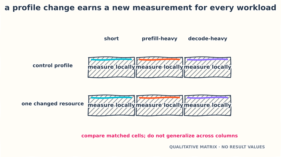
Figure 9. A profile change earns separate measurements for each workload class.

Some rules that survived the Qwen campaign:

• Lowering maximum context can release some runtime memory, but it cannot make an already admitted long prompt cheaper.
• A larger shared token pool helps only when token pages bind before latency or another state pool.
• More recurrent entries need matching graph coverage and workspace.
• Capturing a batch shape avoids a fallback; it does not guarantee the shape satisfies the SLO.
• Smaller prefill chunks can reduce decode stalls and add scheduling overhead. The useful value depends on the mixed workload.
• Prefix reuse can improve TTFT and concentrate traffic on one replica. Measure the router and cache together.
• A speculative mode changes accepted tokens per verification cycle and state use. Qualify it on realistic prompts, not only random token IDs that make the draft structurally unhelpful.

Part IX: Validate load and model behavior separately

First, prove the load test was real

For every retained trial I require:

1. the expected number of measured records;
2. unique warmup prompts excluded from the measured set;
3. the expected measured prompt identities;
4. HTTP success and no cancellation or client timeout;
5. non-empty reasoning_content or content deltas in the SSE stream;
6. final server usage with the requested completion length;
7. the expected finish reason;
8. zero aggregate errors and output-length mismatches;
9. achieved concurrency or offered rate consistent with the test;
10. no fatal server, rank, allocator, or device event in the run window.

I use --use-server-token-count because converting reconstructed text back into tokens does not always invert the server tokenizer exactly. I still inspect the raw stream because a usage counter without generated text is not a useful response. Fast failure is not capacity.

Then, prove the server still behaves like the model

The saturation corpus is not a semantic evaluation. Beside it I keep a small canary suite with normal EOS behavior:

• deterministic factual and reasoning prompts;
• structured output against a schema;
• tool calls and parser behavior;
• thinking and content channel handling;
• multi-turn continuity and repeated prefixes;
• a boundary-length request;
• image input when the deployed profile claims multimodal support.

I compare topology and optimization candidates against the control output where determinism permits. For quantized or speculative paths I use appropriate task checks rather than demand universal byte identity. The canary catches a class of failure that latency records cannot: the endpoint can stream the right number of tokens through the wrong model path.

Part X: Qualify the production envelope

Homogeneous rows are diagnostic, not additive

A short-only boundary and a long-only boundary do not add up to a mixed-server capacity. A long prefill can delay the first token of short work. A long decode can retain scheduler, KV, and recurrent-state resources while new prompts arrive. Prefix reuse changes both compute and routing locality.

A mixed workload must preserve:

class proportions and coupled input/output lengths
session turns and prefix reuse
arrival process by class
per-class SLO vector and priority
tool and structured-output behavior
cancellations, retries, and timeouts
routing and cache-locality policy

I run each class alone to understand its fingerprint, then the traced mix, then stress variants: prefix reuse disabled, burstier arrivals, one replica draining, and cold-cache recovery. I avoid a Cartesian product of independent input and output bins when those pairs do not exist in real traffic.

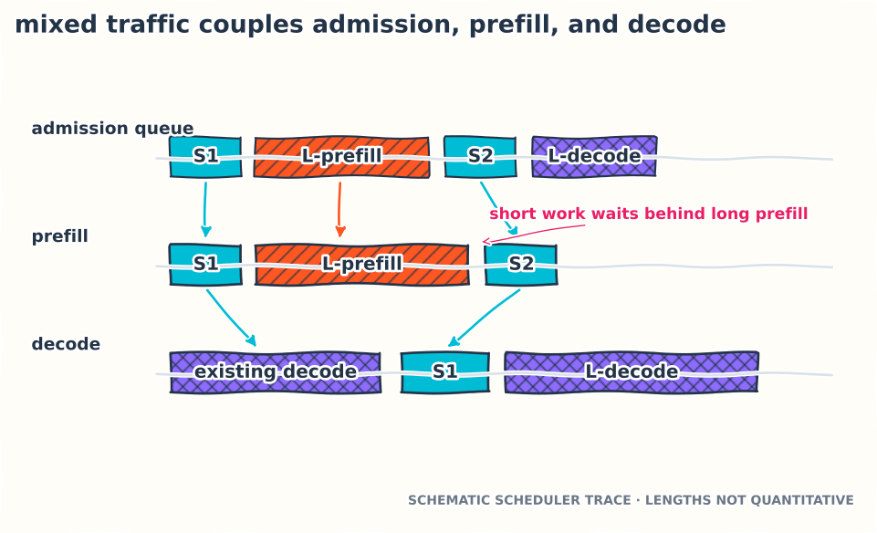
Figure 10. Mixed traffic creates interference that homogeneous boundaries cannot be added to predict.

Research systems such as Llumnix show why heterogeneity and runtime imbalance matter across replicas. I do not need live migration to learn the lesson: per-replica queues, request state, cache locality, and tail latency belong in the capacity model.

The measured edge is not the operating limit

I express production headroom symbolically:

\[ \lambda_{op}(W)=H(W)\,\lambda_{edge}(W,S),\qquad 0<H(W)<1. \]

\(H\) is not a universal safety factor. I derive it from run-to-run variation, arrival burstiness, workload drift, rolling deployment, telemetry overhead, cold-cache recovery, and the failure policy. For replicas I also ask the N-minus-one question: while one replica is draining or unhealthy, do the remaining replicas still meet the mixed-workload contract?

If one qualified replica carries offered rate \(q\) under the chosen contract, a first replica-count estimate is:

\[ R=\left\lceil\frac{\lambda_{peak}}{Hq}\right\rceil. \]

That equation starts the topology discussion. Router imbalance, cache locality, replica interference, and N-minus-one replay decide whether the integer is actually enough.

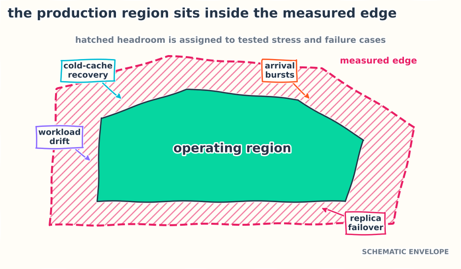
Figure 11. Headroom is evidence from declared failure and drift cases, not a copied percentage.

The retained capacity record belongs to this complete tuple:

(image and model identity, hardware and topology, runtime flags,
 workload distribution, cache state, arrival process, routing policy,
 SLO vector, validity gates, measured edge, headroom evidence)

I requalify it after a model or quantization change, runtime or driver update, topology or routing change, context or state-pool change, graph-policy change, traffic drift, or SLO change.

Fit the real state, separate phase costs, choose TP and replicas on a fixed device budget, keep EP for MoE, use AIPerf to find the neighborhood, certify adjacent points independently, and then challenge the winner with open-loop mixed traffic and failure headroom. That is the capacity plan I can defend when the workload changes.